Guest Post: Lance Dixon on Calculating Amplitudes

This year’s Sakurai Prize of the American Physical Society, one of the most prestigious awards in theoretical particle physics, has been awarded to Zvi Bern, Lance Dixon, and David Kosower “for pathbreaking contributions to the calculation of perturbative scattering amplitudes, which led to a deeper understanding of quantum field theory and to powerful new tools for computing QCD processes.” An “amplitude” is the fundamental thing one wants to calculate in quantum mechanics — the probability that something happens (like two particles scattering) is given by the amplitude squared. This is one of those topics that is absolutely central to how modern particle physics is done, but it’s harder to explain the importance of a new set of calculational techniques than something marketing-friendly like finding a new particle. Nevertheless, the field pioneered by Bern, Dixon, and Kosower made a splash in the news recently, with Natalie Wolchover’s masterful piece in Quanta about the “Amplituhedron” idea being pursued by Nima Arkani-Hamed and collaborators. (See also this recent piece in Scientific American, if you subscribe.)

I thought about writing up something about scattering amplitudes in gauge theories, similar in spirit to the post on effective field theory, but quickly realized that I wasn’t nearly familiar enough with the details to do a decent job. And you’re lucky I realized it, because instead I asked Lance Dixon if he would contribute a guest post. Here’s the result, which sets a new bar for guest posts in the physics blogosphere. Thanks to Lance for doing such a great job.

—————————————————————-

“Amplitudes: The untold story of loops and legs”

Sean has graciously offered me a chance to write something about my research on scattering amplitudes in gauge theory and gravity, with my longtime collaborators, Zvi Bern and David Kosower, which has just been recognized by the Sakurai Prize for theoretical particle physics.

In short, our work was about computing things that could in principle be computed with Feynman diagrams, but it was much more efficient to use some general principles, instead of Feynman diagrams. In one sense, the collection of ideas might be considered “just tricks”, because the general principles have been around for a long time. On the other hand, they have provided results that have in turn led to new insights about the structure of gauge theory and gravity. They have also produced results for physics processes at the Large Hadron Collider that have been unachievable by other means.

The great Russian physicist, Lev Landau, a contemporary of Richard Feynman, has a quote that has been a continual source of inspiration for me: “A method is more important than a discovery, since the right method will lead to new and even more important discoveries.”

The work with Zvi and David, which has spanned two decades, is all about scattering amplitudes, which are the complex numbers that get squared in quantum mechanics to provide probabilities for incoming particles to scatter into outgoing ones. High energy physics is essentially the study of scattering amplitudes, especially those for particles moving very close to the speed of light. Two incoming particles at a high energy collider smash into each other, and a multitude of new, outgoing particles can be created from their relativistic energy. In perturbation theory, scattering amplitudes can be computed (in principle) by drawing all Feynman diagrams. The first order in perturbation theory is called tree level, because you draw all diagrams without any closed loops, which look roughly like trees. For example, one of the two tree-level Feynman diagrams for a quark and a gluon to scatter into a W boson (carrier of the weak force) and a quark is shown here.

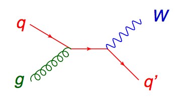
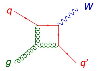
We write this process as qg → Wq. To get the next approximation (called NLO) you do the one loop corrections, all diagrams with one closed loop. One of the 11 diagrams for the same process is shown here.

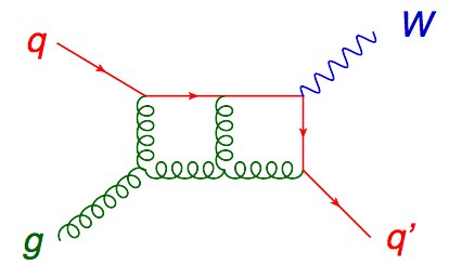
Then two loops (one diagram out of hundreds is shown here), and so on.

The forces underlying the Standard Model of particle physics are all described by gauge theories, also called Yang-Mills theories. The one that holds the quarks and gluons together inside the proton is a theory of “color” forces called quantum chromodynamics (QCD). The physics at the discovery machines called hadron colliders — the Tevatron and the LHC — is dominantly that of QCD. Feynman rules, which assign a formula to each Feynman diagram, have been known since Feynman’s work in the 1940s. The ones for QCD have been known since the 1960s. Still, computing scattering amplitudes in QCD has remained a formidable problem for theorists.

Back around 1990, the state of the art for scattering amplitudes in QCD was just one loop. It was also basically limited to “four-leg” processes, which means two particles in and two particles out. For example, gg → gg (two gluons in, two gluons out). This process (or reaction) gives two “jets” of high energy hadrons at the Tevatron or the LHC. It has a very high rate (probability of happening), and gives our most direct probe of the behavior of particles at very short distances.

Another reaction that was just being computed at one loop around 1990 was qg → Wq (one of whose Feynman diagrams you saw earlier). This is another copious process and therefore an important background at the LHC. But these two processes are just the tip of an enormous iceberg; experimentalists can easily find LHC events with six or more jets (http://arxiv.org/abs/arXiv:1107.2092, http://arxiv.org/abs/arXiv:1110.3226, http://arxiv.org/abs/arXiv:1304.7098), each one coming from a high energy quark or gluon. There are many other types of complex events that they worry about too.

A big problem for theorists is that the number of Feynman diagrams grows rapidly with both the number of loops, and with the number of legs. In the case of the number of legs, for example, there are only 11 Feynman diagrams for qg → Wq. One diagram a day, and you are done in under two weeks; no problem. However, if you want to do instead the series of processes: qg → Wqg, qg → Wqgg, qg → Wqggg, qg → Wqgggg, you face 110, 1253, 16,648 and 256,265 Feynman diagrams. That could ruin your whole decade (or more). [See the figure; the ring-shaped blobs stand for the sum of all one-loop Feynman diagrams.]

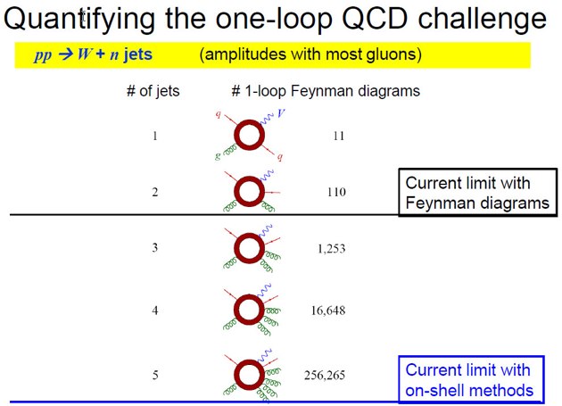
It’s not just the raw number of diagrams. Many of the diagrams with large numbers of external particles are much, much messier than the 11 diagrams for qg → Wq. Plus the messy diagrams tend to be numerically unstable, causing problems when you try to get numbers out. This problem definitely calls out for a new method.

Why care about all these scattering amplitudes at all? Well they, plus many other processes, go into the grand corpus of Standard Model predictions at the LHC. Without a precise knowledge of “old” Standard Model physics, experimenters would have more trouble looking for any “new physics” that might sit on top of it. And many types of new physics can generate multiple jets. Heavy new particles are expected to decay rapidly into a number of light particles, including the quarks and gluons that make jets.

But back to 1990. Around then, nobody could contemplate computing loop amplitudes with 1000 Feynman diagrams, let along hundreds of thousands. Zvi and David had the insight that superstring theory could be used to reorganize perturbation theory in a better way than Feynman diagrams, by taking a limit to get rid of all the unwanted string states. They demonstrated their method on the one loop amplitude for gg → gg, which had been computed using Feynman diagrams a few years earlier by Keith Ellis and James Sexton. Zvi and David got the same result, and they also broke it up into somewhat simpler pieces. But the true test of a good technique is to do something that hasn’t been done by previous methods. Zvi, David and I set out to do a five-leg process, gg → ggg.

We knew the formulas were likely to be more complicated, because the answer could depend on more energies and angles. The four-leg process depends on only two variables, the overall energy and the scattering angle. But the five-leg process depends on five such variables. You can build much more complicated analytic functions out of five variables than just two. Nevertheless, we managed to complete the calculation of the one-loop gg → ggg amplitude, and simplify it down as much as possible.

Then we stared at it. This was the really important part. You can stare at it too.

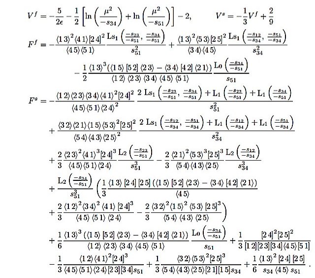
It might look like gibberish to you, but every term in the analytic formula for the gg → ggg scattering amplitude told us something. Every factor in the denominator of the different terms told us exactly how the amplitude “degenerated” (became large) when two of the gluons were pointing in the same direction. Every “L” and “Ls” function told us something else too, which we’ll get to in a second. Fortunately, the expression had exactly the right amount of complexity — not too simple and yet not too horrendously complicated — so that just by staring at it, the various “moving parts” in it started to reveal to us the rules by which it, and other amplitudes, should be put together.

Instead of using Feynman diagrams, or even the string-based diagrammatic rules that Zvi and David had invented, we, together with Dave Dunbar, realized that we could apply a more general and simple principle called unitarity, in order to assemble the amplitude essentially from scratch. Unitarity is roughly the statement that the sum of the probabilities of all possible occurrences is one. In the case of scattering amplitudes, it says that you can get loop amplitudes by sewing together tree amplitudes that live on opposite sides of a line, called a unitarity cut. The legs that cross the cut have to be summed over (like summing over probabilities). See the figure.

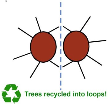
This figure also shows that the method is “environmentally correct” — which is important here in California — since it recycles trees into loops. Efficient recycling would be important later.

For one loop amplitudes, we just needed to multiply together two very simple tree amplitudes, joined by two lines crossing the cut. First of all, that rule explained to us why certain L and Ls functions didn’t appear. Even better, with a little algebra, we found we could recover all the terms containing the L and Ls functions. For the simple tree amplitudes, we relied on previous advances made in the 1980s by Stephen Parke, Tom Taylor, T.T. Wu, Fritz Berends, Walter Giele, Zoltan Kunszt, Michelangelo Mangano, James Stirling, Zhan Xu, Da-Hua Zhang, Lee Chang, and others. In particular, Parke and Taylor had found a remarkable infinite sequence of tree-level amplitudes which we used, along with closely related tree amplitudes.

Actually there was one part we couldn’t get quite so simply at first, the “rational part”, which didn’t have any L’s or Ls’s in it. So, like good theorists, we just changed the theory for a little while, in order to make that part go away. We dropped our study of QCD amplitudes temporarily, and switched to studying its favorite cousin (among hep-th theorists), N=4 super-Yang-Mills theory. For this gauge theory we found that we could work out not just the five-leg process, but one-loop amplitudes with an arbitrarily large number of external gluons (if their spins were pointing the right way). These were the one-loop versions of the Parke-Taylor amplitudes. And we could do it all with exactly the same few-line calculation. That was the beginning of the “unitarity method”. It merged the general principles of unitarity with a certain framework coming from perturbation theory (a known form for loop integrals) in order to determine “the loop integrand”. From simple trees we could get simple loops.

Later, Zvi, David and I figured out how to make the unitarity method somewhat more efficient, and to determine that missing rational part for more QCD processes, like qg → Wqg which we computed back in 1997. For that case, the full result was as simple as it could possibly be made, yet it was still dozens of pages of mind-numbing, eye-straining formulas. We knew then that to go further, we would need to develop a general algorithm that we could automate and computerize. We needed to industrialize, and yet we only had tools for artisan work. So we took a break from this research direction for a while.

In 2003, Ed Witten invented twistor string theory, building in part off foundations laid in the 1960s by Roger Penrose, and in 1988 by Parameswaran Nair. Twistor string theory (in very brief) is a way of getting QCD directly from string theory without having to take any limits. Smart young physicists like Ruth Britto, Freddy Cachazo, Bo Feng, Radu Roiban, Mark Spradlin and Anastasia Volovich flooded what had been a mostly deserted “amplitudes” landscape. They brought new insights about the analytic structure of the loop integrand, such as the importance of something called the quadruple cut. The first three, and Witten, found the BCFW recursion relations (http://arxiv.org/abs/hep-th/0412308, http://arxiv.org/abs/hep-th/0501052). These relations are for tree amplitudes, but they embody the idea that amplitudes should be thought of as plastic, deformable, fluid objects, which can be deformed until they split into pieces. The knowledge of exactly how they split into pieces can be used to construct the tree amplitudes recursively.

In some sense, Feynman diagrams are like grains of sand. If your process needs only a few of them, then they are very useful building blocks and each one holds physical significance. But once you get to thousands, or hundreds of thousands of them for a given process, a kind of phase transition takes place: individual diagrams cease to have any meaning, and you should think of the amplitude as flowing smoothly, like a handful of sand flows through your fingers.

This fluid picture is also inspired by string theory. String theory replaces all Feynman diagrams with a single rubbery surface at each loop order, and you can think of the surface as deforming smoothly as the energies and angles of the particles vary.

Zvi, David and I realized that similar ideas that led to the BCFW recursion relations would also work to automatize the one-loop problem, both for systematically picking apart the unitarity cuts, and for one method to get the missing rational part. We were joined by some remarkable postdocs: Carola Berger, Giovanni Diana, Fernando Febres Cordero, Darren Forde, Tanju Gleisberg, Harald Ita and Daniel Maitre, and more recently Stefan Hoeche. Without them we could never have developed these ideas into a form suitable for automatic evaluation, leading to the “BlackHat” program for computing QCD amplitudes for the LHC.

By now, we were certainly not the only ones working in this direction. Other related ideas and algorithms were developed by Giovanni Ossola, Costas Papadopoulos and Roberto Pittau (http://arxiv.org/abs/hep-ph/0609007, http://arxiv.org/abs/arXiv:0802.1876); and by Keith Ellis, Walter Giele, Zoltan Kunszt, Kirill Melnikov and Giulia Zanderighi (http://arxiv.org/abs/arXiv:0708.2398, http://arxiv.org/abs/arXiv:0810.2762, http://arxiv.org/abs/arXiv:1105.4319). (And many others later on). This was the beginning of the “NLO revolution”, around 2007-2010. Inspired also by the needs (or “wish lists”) of experimentalists, including constant cheerleading by Joey Huston, the community went from a barren handful of 2 → 3 LHC processes known at NLO, to a full cornucopia of 2 → 4 processes, and eventually even a few 2 → 5 and 2 → 6 processes. Some of the modern methods are not purely unitarity based, but most of them have strong similarities. In the automated programs they spawned, the ability to recycle simpler building blocks is the key to computing amplitudes fast enough to get reliable results. (Certain theoretical errors are statistical, and can only be beaten down by evaluating the same answer many times, for many different particle energies and angles.) Having a speedy method is of the essence, but it also helps to have a lot of computer power at your disposal!

There have been plenty of other applications of these methods, often farther from experiment. Zvi, David and I have been especially interested in applying them to theories with a lot of supersymmetry, including N=4 super-Yang-Mills theory (the most supersymmetric gauge theory) and N=8 supergravity (the most supersymmetric theory of gravity). The supersymmetry makes it possible to recognize patterns and go to much higher loop order than we can presently do in QCD. I’ll be briefer here because you, the reader, must be getting tired by now.

While N=4 super-Yang-Mills theory is very special, it gets even more special when the number of colors is large. In this limit, the famous AdS/CFT correspondence, which relates the strong-coupling limit to a theory of gravity, is the most manifest. In 2003, Babis Anastasiou, Zvi, David and I used unitarity and inspected the two-loop amplitude in this theory and realized it had a special “iterative” property. In 2005, Zvi, Volodya Smirnov and I went on to three loops — using the unitarity method and Volodya’s wizardry with loop integrals. With the additional patterns we could see emerging at three loops, we could make a stronger conjecture, that the amplitudes would obey a perfect exponential pattern. Actually our conjecture was a bit too strong; only the four and five-leg amplitudes work this way. It later transpired that those amplitudes work because they are fixed by a secret symmetry, called dual conformal symmetry. This symmetry has its roots in work by David Broadhurst and Lev Lipatov in the 1990’s; its appearance was recognized in the N=4 loop integrands by James Drummond, Johannes Henn, Emery Sokatchev and Volodya Smirnov around 2006.

Zvi and I convinced Juan Maldacena, one of the inventors of the AdS/CFT correspondence, to try to use that correspondence to compute N=4 scattering amplitudes at strong coupling and test our conjecture. He and Fernando Alday did so, first for the four-gluon amplitude, and they found complete agreement with our prediction. They made use of an exact result by Niklas Beisert, Burkhardt Eden and Matthias Staudacher (BES) for the divergent part of the amplitude (the so-called cusp anomalous dimension). Alday and Maldacena also gave an explanation for why dual conformal symmetry appears, and many other hints to help understand the weak coupling (perturbative) side.

We now have a hope that we can solve exactly for all the scattering amplitudes in this theory. Part of this hope is pinned on new formulations for the multi-loop integrand being developed by Nima Arkani-Hamed and his collaborators — such as the “amplituhedron” (which I won’t explain here!). Another part of the hope (for me) is pinned on recent work by Benjamin Basso, Amit Sever and Pedro Vieira. That work relates certain limits of N=4 amplitudes (via polygonal Wilson loops, but that’s another story) to exact scattering matrices of a certain two-dimensional theory. Their work is closely related to the framework BES used for the divergent part, and involves some bold conjectures, but we have been testing their predictions through three and four loops (in work with James Drummond, Claude Duhr, Matt von Hippel, and Jeff Pennington) and every prediction pans out perfectly so far.

Finally, let me mention N=8 supergravity. This theory was invented by Eugene Cremmer and Bernard Julia in the late 1970s, with other important contributions from Bernard deWit and Hermann Nicolai, Joel Scherk and others. When superstring theory had its 1984 revolution, N=8 supergravity was quickly pronounced dead — because string theory was manifestly free of all ultraviolet divergences, and how could any point-particle theory dare to make that claim? However, it never received a proper burial. At that time, it was generally thought that N=8 supergravity would diverge at three loops, but no-one could do a full calculation past one loop. With the unitarity method, we could get to two loops in 1998 (with Zvi, Dave Dunbar, Maxim Perelstein and Joel Rozowsky), to three loops in 2007 (with Zvi, David, John Joseph Carrasco, Henrik Johansson and Radu Roiban), and to four loops in 2009. We still have found no direct sign of a divergence in N=8 supergravity, although the conventional wisdom has retreated from a first divergence at three loops to a first one at seven or eight loops. Zvi, John Joseph, Henrik and Radu are pushing ahead to five loops, which will also give important indications about seven loops. A first divergence at even the seven loop order would be the smallest infinity known to man…

Along the way, Zvi, John Joseph and Henrik, thanks to the time-honored method of “just staring at” the loop integrand provided by unitarity, also stumbled on a new property of gauge theory amplitudes, which tightly couples them to gravity. They found that gauge theory amplitudes can be written in such a way that their kinematic part obeys relations that are structurally identical to the Jacobi identities known to fans of Lie algebras. This so-called color-kinematics duality, when achieved, leads to a simple “double copy” prescription for computing amplitudes in suitable theories of gravity: Take the gauge theory amplitude, remove the color factors and square the kinematic numerator factors. Crudely, a graviton looks very much like two gluons laid on top of each other. If you’ve ever looked at the Feynman rules for gravity, you’d be shocked that such a simple prescription could ever work, but it does. Although these relations could in principle have been discovered without unitarity-based methods, the power of the methods to provide very simple expressions, led people to find initial patterns, and then easily test the patterns in many other examples to gain confidence.

Nowadays, there is a boom in “amplitudes” research — research devoted to understanding the analytic behavior and remarkable structures present in scattering amplitudes and then turning that knowledge into new methods. There is an annual “Amplitudes” meeting, as well as many other related workshops. Landau’s maxim has been a recurrent one throughout the field, and itself has been applied recursively: new methods lead to discoveries, which lead to newer methods, which lead to even more discoveries, ad infinitum. There’s a remarkable richness and beauty to scattering amplitudes, which every researcher perceives differently, but which attracts them all to the field.