Ken Wilson, Nobel Laureate and deep thinker about quantum field theory, died last week. He was a true giant of theoretical physics, although not someone with a lot of public name recognition. John Preskill wrote a great post about Wilson’s achievements, to which there’s not much I can add. But it might be fun to just do a general discussion of the idea of “effective field theory,” which is crucial to modern physics and owes a lot of its present form to Wilson’s work. (If you want something more technical, you could do worse than Joe Polchinski’s lectures.)
So: quantum field theory comes from starting with a theory of fields, and applying the rules of quantum mechanics. A field is simply a mathematical object that is defined by its value at every point in space and time. (As opposed to a particle, which has one position and no reality anywhere else.) For simplicity let’s think about a “scalar” field, which is one that simply has a value, rather than also having a direction (like the electric field) or any other structure. The Higgs boson is a particle associated with a scalar field. Following the example of every quantum field theory textbook ever written, let’s denote our scalar field φ(x, t).
What happens when you do quantum mechanics to such a field? Remarkably, it turns into a collection of particles. That is, we can express the quantum state of the field as a superposition of different possibilities: no particles, one particle (with certain momentum), two particles, etc. (The collection of all these possibilities is known as “Fock space.”) It’s much like an electron orbiting an atomic nucleus, which classically could be anywhere, but in quantum mechanics takes on certain discrete energy levels. Classically the field has a value everywhere, but quantum-mechanically the field can be thought of as a way of keeping track an arbitrary collection of particles, including their appearance and disappearance and interaction.
So one way of describing what the field does is to talk about these particle interactions. That’s where Feynman diagrams come in. The quantum field describes the amplitude (which we would square to get the probability) that there is one particle, two particles, whatever. And one such state can evolve into another state; e.g., a particle can decay, as when a neutron decays to a proton, electron, and an anti-neutrino. The particles associated with our scalar field φ will be spinless bosons, like the Higgs. So we might be interested, for example, in a process by which one boson decays into two bosons. That’s represented by this Feynman diagram:
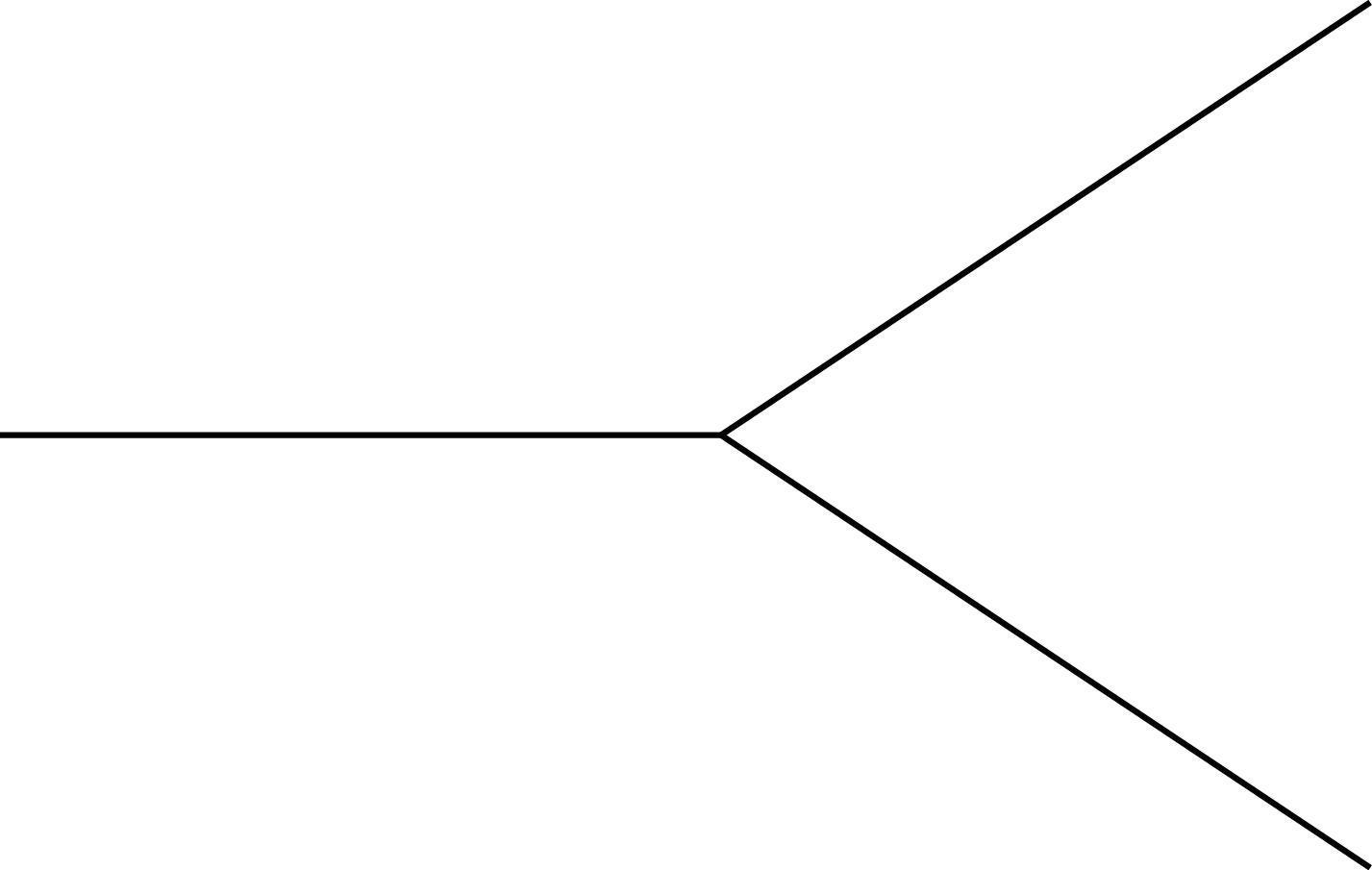
Think of the picture, with time running left to right, as representing one particle converting into two. Crucially, it’s not simply a reminder that this process can happen; the rules of quantum field theory give explicit instructions for associating every such diagram with a number, which we can use to calculate the probability that this process actually occurs. (Admittedly, it will never happen that one boson decays into two bosons of exactly the same type; that would violate energy conservation. But one heavy particle can decay into different, lighter particles. We are just keeping things simple by only working with one kind of particle in our examples.) Note also that we can rotate the legs of the diagram in different ways to get other allowed processes, like two particles combining into one.
This diagram, sadly, doesn’t give us the complete answer to our question of how often one particle converts into two; it can be thought of as the first (and hopefully largest) term in an infinite series expansion. But the whole expansion can be built up in terms of Feynman diagrams, and each diagram can be constructed by starting with the basic “vertices” like the picture just shown and gluing them together in different ways. The vertex in this case is very simple: three lines meeting at a point. We can take three such vertices and glue them together to make a different diagram, but still with one particle coming in and two coming out.
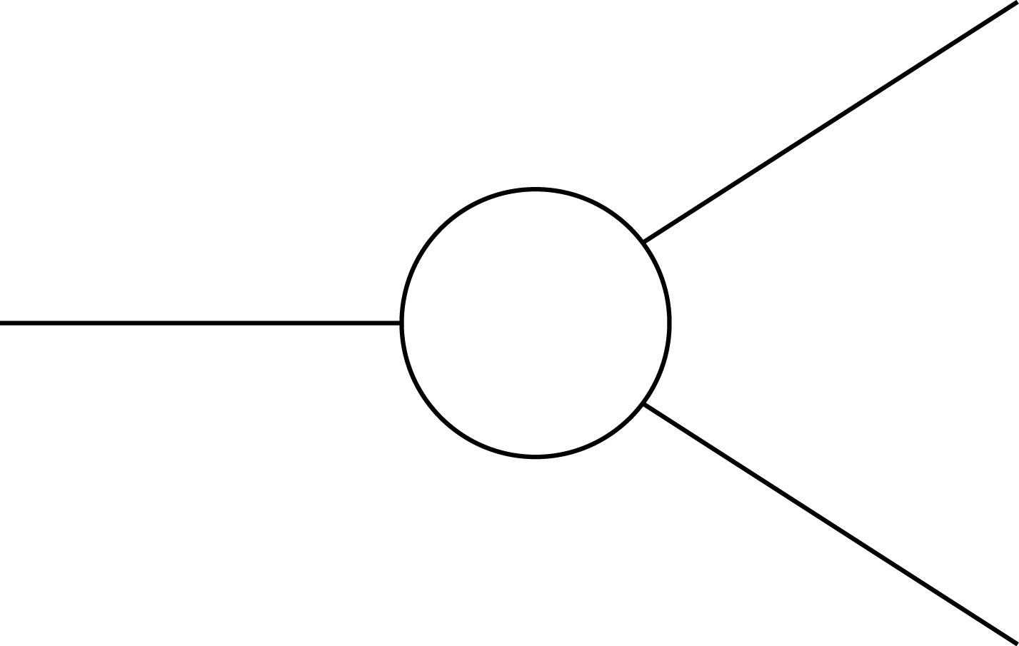
This is called a “loop diagram,” for what are hopefully obvious reasons. The lines inside the diagram, which move around the loop rather than entering or exiting at the left and right, correspond to virtual particles (or, even better, quantum fluctuations in the underlying field).
At each vertex, momentum is conserved; the momentum coming in from the left must equal the momentum going out toward the right. In a loop diagram, unlike the single vertex, that leaves us with some ambiguity; different amounts of momentum can move along the lower part of the loop vs. the upper part, as long as they all recombine at the end to give the same answer we started with. Therefore, to calculate the quantum amplitude associated with this diagram, we need to do an integral over all the possible ways the momentum can be split up. That’s why loop diagrams are generally more difficult to calculate, and diagrams with many loops are notoriously nasty beasts.
This process never ends; here is a two-loop diagram constructed from five copies of our basic vertex:
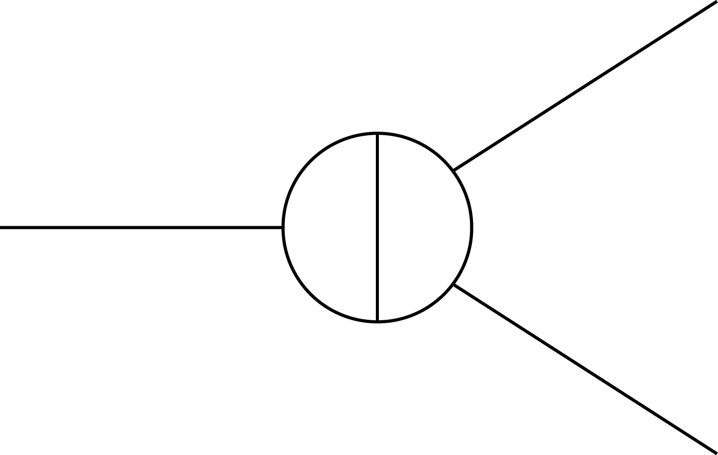
The only reason this procedure might be useful is if each more complicated diagram gives a successively smaller contribution to the overall result, and indeed that can be the case. (It is the case, for example, in quantum electrodynamics, which is why we can calculate things to exquisite accuracy in that theory.) Remember that our original vertex came associated with a number; that number is just the coupling constant for our theory, which tells us how strongly the particle is interacting (in this case, with itself). In our more complicated diagrams, the vertex appears multiple times, and the resulting quantum amplitude is proportional to the coupling constant raised to the power of the number of vertices. So, if the coupling constant is less than one, that number gets smaller and smaller as the diagrams become more and more complicated. In practice, you can often get very accurate results from just the simplest Feynman diagrams. (In electrodynamics, that’s because the fine structure constant is a small number.) When that happens, we say the theory is “perturbative,” because we’re really doing perturbation theory — starting with the idea that particles usually just travel along without interacting, then adding simple interactions, then successively more complicated ones. When the coupling constant is greater than one, the theory is “strongly coupled” or non-perturbative, and we have to be more clever.
So far, so good. Now for the bad news. In many cases of interest, when we actually do the integral over momentum in the loop diagrams, we get an answer that is not at all small, even when multiplied by appropriate powers of the coupling constant — in fact, the answer can be infinite! Generally a sign that something has gone terribly wrong.
The great contribution of Feynman, Schwinger, Tomonaga, and Dyson was to show that we didn’t necessarily have to despair at this apparent disaster: certain quantum field theories can be “renormalized” to get sensible answers. Renormalization has gained a reputation as being somewhat mysterious, perhaps even disreputable, but it’s really not a big deal: it’s just a matter of taking a limit in a careful way so that we get finite answers for perfectly reasonable physical questions. One of Wilson’s great contributions was to make the physical meaning of renormalization more clear.
Let’s think a bit about why the loop diagrams are giving infinite answers — why, as we say, they are divergent. It’s because we were integrating (summing) over all the possible ways that momentum could move through the loops. And in particular, on closer inspection, the divergences arise from allowing the momentum to get arbitrarily large. Momentum is a vector, so even if a finite amount comes into the loop, we can always divide it into an arbitrarily large amount going one way and a similarly large amount pointing in the opposite physical direction, so the sum is constant. But if you think about it, “large momentum” corresponds to “high energies” or (in quantum mechanics) “short distances.” And it’s at high energies/short distances where all sorts of funny things can be lurking — from new kinds of particles we haven’t yet discovered (and therefore don’t include in our Feynman diagrams) to a breakdown of spacetime itself. So maybe we shouldn’t expect this sum over arbitrarily large momenta to give any sensible answers.
Is it possible to do useful work in quantum field theory without worrying about the “ultraviolet” (high-energy, short-distance) regime? Yes it is, says Ken Wilson: we can talk about an “effective field theory” that is only valid below some energy scale, in which case what goes on at high energies is simply irrelevant. And thus he made quantum field theory safe for the world.
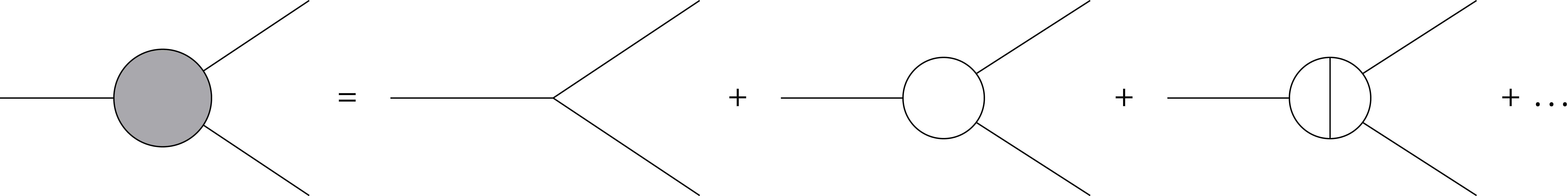
Let me explain what this means, although I’ll do it in a somewhat non-Wilsonian way. (I’m going to talk about diagrams, Wilson would take a path integral over all the quantum fields and divide things up into high energies and low energies.) Remember that what we are using our quantum field theory for is to calculate the rate at which particles interact with each other in various ways. For example, we’ve been looking at one particle decaying into two. That’s a sum of an infinite number of Feynman diagrams, including loops with arbitrarily large momenta inside. But let’s forget about the details, and just think about the final answer. We can express that answer (whatever it turns out to be) as a “blob diagram,” which morally represents the sum of all the real Feynman diagrams.
Likewise for other processes we might be interested in. For example, our theory will allow two bosons to scatter off each other into two more bosons, which we can represent diagramatically as well.
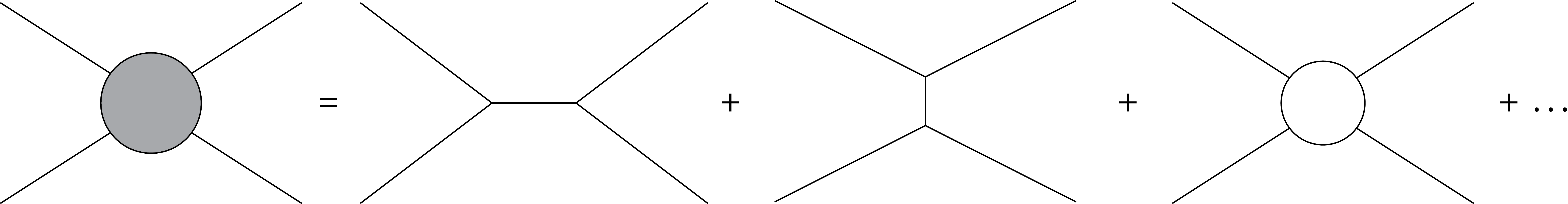
So far this is just re-writing our ignorance in a convenient way. What Wilson says is that we don’t need to know what is actually going on at arbitrarily high energies, which would correspond to the high-momentum contributions from the diagrams on the right. Instead, there is a different theory — the effective theory — that simply encapsulates the blob diagrams on the left. If we knew the true theory, we could derive the effective theory by actually integrating over all those loops with large momenta moving through them. But the beauty is that we don’t need to know the true theory — we are welcome to work with the effective theory in its own right. Indeed, there can be many possible “true” theories — many “ultraviolet completions” — that would give you exactly the same low-energy effective theory!
The good news is, we can usefully do quantum field theory without knowing absolutely everything about nature. The bad news is, it can be very hard to figure out what nature is actually doing at very high energies, since it’s all bundled up in an effective field theory. That’s why it’s hard to test something like string theory at the LHC. As Polchinski says, “Nobody ever promised you a rose garden.”
The nice thing about all this is that effective field theories are really quite “effective.” That is, they are not arbitrarily complicated; it’s generally quite simple to figure out what processes are important and which ones are less so.
To see this all we need (he says, chuckling maniacally) is a bit of dimensional analysis. We’ll use natural units, in which Planck’s constant ℏ and the speed of light c are both set equal to unity. In natural units, everything can be expressed as different powers of a single kind of quantity. We will choose “energy” as our measuring stick, in which case we have:
Mass = Energy; Length = 1/Energy; Time = 1/Energy.
(If you’ve never seen this before, and don’t mind a bit of arithmetic, it’s worth checking that these follow from setting ℏ=c=1.)
So what are the units of our field φ? Well, vibrations in the field carry energy. We talk about the “kinetic energy density,” which is just the amount of kinetic energy the field carries in any specified volume of space. If the “velocity” of the field is its time derivative dφ/dt, the kinetic energy density is

If you’ve never seen this formula before, I’m just pulling it out of thin air; but notice that it bears a family resemblance to the kinetic energy of a particle, (1/2)mv2, since the velocity is the time derivative of the position.
The left-hand side here has units of energy/volume; volume has units of length3; and length has units of 1/energy. So the left side has units of energy4, and therefore so does the right-hand side. The time derivative d/dt has units of 1/time, which is the same as energy; and its squared, so that’s energy2. All that’s left (since 1/2 is a dimensionless number) is the field, which is also squared. To make left and right match, the field must have units of energy:
[φ] = energy.
Awesome. Now, in quantum field theory, each of the blob diagrams above corresponds to a quantum “operator”; there’s an operator that connects three particles (e.g. by taking one particle into two), one that connects four particles (e.g. by taking one into three, or two into two, etc.), and so on. Each operator has a dimension, which we can figure out by dimensional analysis. (Technical note: in addition to the field itself, operators can also involve derivatives of the field. Derivatives have units of 1/length or 1/time, i.e. units of energy. We’re just ignoring this possibility.)
The three-particle operator (corresponding to the diagram with three lines coming into the blob) must have the dimensions of our original three-particle vertex (since that’s one of the terms that sums to get the blob). If you dig into the equations of field theory, that’s just the field itself raised to the third power. (Likewise a four-particle vertex would be the field to the fourth power, etc. — each appearance of the field in the expression from which the vertex derives corresponds to one line coming into or out of the vertex.) So the dimension of that three-point blob is equal to that of φ3, which is of course just energy3. Every operator (every blob diagram) has units of energy to some power, so all that matters is what that power is. If the power is three, we say we have a “dimension-three operator.” Our four-particle blob is a dimension-four operator, and so on. (Yes, I know, a lot of work just to say “the dimension of the blob is the number of lines coming in/out.” In other theories it would be more complicated. The electron field, for example, is a fermion rather than a boson, and it turns out to have dimensions energy3/2, so a diagram with four electron lines is dimension-6.)
Honestly there is a reason we’re going through all this. Each of those blob diagrams represents something that could happen at some point in spacetime. The chance that it happens anywhere is obtained by integrating all over spacetime. This quantity (really we’re talking about terms in the effective action) therefore has units of spacetime volume times the units of our operator. And spacetime volume has units of 1/energy4 (sticking with good old four-dimensional spacetime). So if we have an operator of dimension N, the thing we really care about — the integral over all of spacetime of our operator, from which we can derive the quantum probability amplitude — has units of
[spacetime integral of operator of dimension N] = energyN-4.
Why do we care about that? Because, once again following Wilson’s logic, the interactions in our effective theory change as we change our definition of “high energy” (the part we’re bundling up) vs. “low energy” (the part we’re explicitly describing in our theory). As we change this “cutoff,” we are including or excluding different processes, thereby altering the effective coupling constants. That change is known as the renormalization group. It spells immediate doom for many crackpotty attempts at unification that try to derive, for example, the fine-structure constant in terms of π and e and the author’s birthday. The coupling constants of an effective field theory are not really constant; they depend on the energy at which you measure them. This can have dramatic consequences. In quantum chromodynamics, the theory of quarks and gluons, the coupling constant is small at high energies and everything is perturbative. But at low energies the coupling becomes strong, and the theory changes character completely — the new effective field theory is one of light bound states (pions), not a theory of quarks and gluons at all.
And this innocent-looking formula, coming from a bit of dimensional analysis, tells us roughly how that change goes. The importance of an operator of dimension N (where N is just the number of particles involved in the blob diagram, in our simple scalar-field-theory example) grows at high energy if its spacetime integral goes as a positive power of energy; i.e., if N>4. But we don’t care about high energies! We are trying to construct an effective theory at low energies, so we care about the terms for which N≤4 — those are the ones that dominate at low energies. In fact, we have lingo to encapsulate this importance. When talking about operators with units of energyN in four spacetime dimensions, we refer to them as:
- N<4: relevant
- N=4: marginal
- N>4: irrelevant
The labels relevant/marginal/irrelevant are telling us how important such operators are to a low-energy effective field theory. (Strictly speaking, even “irrelevant” operators can be important. In the Fermi theory of the weak interactions, the lowest-order operator you can construct that gives rise to any interaction at all is dimension 6. So you have to keep that interaction to have anything interesting happen — but we say that the resulting theory is “non-renormalizable.”) (And while we’re speaking strictly, this dimensional analysis gives the leading behavior, but not the whole story. In QCD, for example, the coupling is marginal, but it doesn’t remain exactly constant with energy, but rather changes slowly [logarithmically]. If all of your couplings are exactly constant, you have a conformal field theory.)
For those few of you who have made it this far, please appreciate how wonderful this is! Above we were drawing Feynman diagrams representing processes in an effective field theory, and we argued that diagrams with N scalar particles coming in and out would have dimension N. And now we’ve seen that, at low energies, the only relevant (and marginally relevant) processes are those with N≤4. But if N is the number of particles involved, it’s going to be a positive integer. And there aren’t that many positive integers less than or equal to four!
In fact, there are only four of them. A one-particle operator would represent a particle disappearing into, or appearing out of, empty space. We don’t think that can happen (energy conservation), so that’s not very important. A two-particle operator just has one particle going in and one particle coming out — i.e., it’s just a particle propagating through space. Indeed, we call it the propagator. And then there are the three-particle and four-particle processes we mentioned above.
And that’s it! Those pieces give you the important low-energy description of any theory of a single scalar field, no matter what new particles and crazy nonsense might be going on at higher energies. Of course we don’t work at strictly zero energy, so the “irrelevant” parts might also be interesting and useful, but Wilsonian effective field theory gives you a systematic way of dealing with them and estimating their importance.
If you have more than one kind of particle/field running around in your theory, there will naturally be more operators to deal with — but still a manageable number of relevant/marginal ones. The effective field theory philosophy tells you to write down all of the relevant and marginal operators consistent with the underlying symmetries of your theory. You can then measure their coefficients in some kind of experiment, and use that data to predict the answer for any other kind of experiment you might want to do. In fact, you’re not allowed to only write down some of the operators consistent with your symmetries; generically we would expect all such operators to be generated by the higher-energy processes we’re ignoring.
Wilson’s viewpoint, although it took some time to sink in, led to a deep shift in the way people thought about quantum field theory. Pre-Wilson, it was all about finding theories that are renormalizable, which are very few in number. (The old-school idea that a theory is “renormalizable” maps onto the new-fangled idea that all the operators are either relevant or marginal — every single operator is dimension 4 or less.) Nowadays we know you can start with just about anything, and at low energies the effective theory will look renormalizable. Which is useful, if you want to calculate processes in low-energy physics; disappointing, if you’d like to use low-energy data to learn what is happening at higher energies. Chances are, if you go to energies that are high enough, spacetime itself becomes ill-defined, and you don’t have a quantum field theory at all. But on labs here on Earth, we have no better way to describe how the world works.
This was awesome. Thank you!
You—and Matt Strassler—do a wonderful public service in your talks and writings. Thank you.
I’d like to compliment your article without disparaging someone else, except I won’t… where’s the fun in that?
Thank you for doing in 10 minutes what an unnamed UofC physics professor could not do in 1 quarter.
Thank you!
Not for the first time, you set a standard for us other science bloggers to aspire to.
Good stuff Sean. Nice to see mention of the fine structure constant being a running constant. But you know how you said “momentum is a vector, so even if a finite amount comes into the loop” along with “the electron field… turns out to have dimensions energy³/²”? That’s because the momentum is in a loop, something like this BEC spinor. Look out for blue toruses on TQFT websites. Methinks there’s going to be some even more effective quantum field theory coming soon.
“A one-particle operator would represent a particle disappearing into, or appearing out of, empty space. We don’t think that can happen (energy conservation), so that’s not very important.”
i guess I’ll be reading up on Ken Wilson and effective field theory for the rest of my break.
Sean, this is so good!
Thank you for taking the time to write this, very interesting!
Glad people like it!
Thank you very much for this. I’ve wondered what renormalization is for a while, this makes it as clear as it will be until I get to this point in school. And will probably help me a lot at that point.
Sean – any chance you will ever write a QFT book, at roughly the level of “Spacetime + Geometry”?
Bob, you never know. But it’s not a high priority right now, and writing a textbook is one of those things that better be a very high priority or it doesn’t get done. So I would say, not in the next ten years. Also, there are dozens of QFT textbooks already written, by people who know the subject much better than I do.
Knowing the subject much better than you does not necessarily qualify someone to write a good QFT book. Communication skills are much more important!
I think this summarizes the entire second semester of my graduate quantum field theory course.
Whoa! You made a blog post longer than a paragraph and without any videos! I am impressed.
Care to recommend any?
Peskin & Schroeder is by now the “standard” textbook, and quite a good one. Zee is also good, but for inspirational purposes more than calculational ones. Srednicki is also very good. (All the good QFT textbooks these days come from California.)
Pingback: Effective Quantum Field Theory | Observer
Thanks for this Sean, it’s one of the clearest “non-technical” explanations I’ve ever read of such a deep idea in Physics.
This is a very nice explanation of Wilson’s work. But my feeling (most likely naïve) is that if you want to calculate some process at low or high energy and compare with experiments, you still have to go through old fashioned field theory calculation (whether it is renormaliazable or not). Also, does Wilson’s method give same answers (exact or approximate) for renormalizable theories where you would include N>4 diagrams. Anyone cares to make comments?
After reading this pristine explanation, I think some professors shall be forbidden eternally from teaching QFT.
In your very fine article, you mentioned the decay of the Neutron into a Proton, Electron and a Positron Neutrino. From what I understand the Neutron is a composite particle. Also, putting neutrons in a particle accelerator and bounce electrons off of them results in scattering events. Analyzing these scattering events shows that there are three different scattering centers inside the Neutron. Therefore, the Neutron is not composed of the Positron Neutrino as its’ mass is too small for scattering. The idea, as I understand, is that the Neutron is composed of 1 up and 2 down quarks. The Proton is composed of 2 up and 1 down quark. Is it also true that the Proton is not seen as a composite particle and does not show three scattering centers? The up and down quarks all have the same mass (360MeV from what I have read) and the Electron and Positron contain no quarks. However, the Neutron has a larger mass than the Proton. The question then is ‘what is the nature of the energy difference between the Proton and the Neutron if the Quarks that compose each particle have the same mass and the Neutron has a larger mass’? You did use the Neutron as your example:)
Thomas: the up and down quarks do not have the same mass. When discussing the mass of the proton and neutron, it also matters which mass you are considering.
The up quark has a “bare mass” of about 2 MeV, while the down quark is about 5 MeV. These numbers are approximate, because we never observe bare quarks: confinement means they are always bound into hadron states, including baryons like the proton and neutron.
When quarks are in these bound states, we can talk about their “effective” or “dressed” masses which take into account the binding energy from gluons. I think that is the source of the “360 MeV” number that you remembered.
The difference in masses between the proton and neutron is related to the difference in bare masses of the up and down quark. However, to my knowledge there is not yet a calculation which explains the difference completely. This is a problem in low-energy quantum chromodynamics, and as Sean mentioned in this blog post, QCD becomes non-perturbative at low energies, making calculations very difficult.
Kevin;
Thank you for your answer; it’s appreciated. I want ask you, or anyone, if anyone knows of any experiment that did a direct measurement of the gravitational attraction between two (frozen in place?) Lithium atoms? I think I remember reading of such an experiment; but, I find no reference. Of course, I could be wrong.
The thought is ‘can the gravitational attraction between two neutral Hydrogen atoms be measured by any conceivable experiment’? Why might I think that neutral Hydrogen is gravitationally unique among the elements and want an atom to atom experimental measurement (as opposed to a calculation from general laws)? read between the lines in the following article. (…the musts and can nots?)
http://www.csmonitor.com/Science/2013/0508/Colossal-hydrogen-bridge-between-galaxies-could-be-fuel-line-for-new-stars/(page)/1