Guest Post: Nicole Yunger Halpern on What Makes Extraordinary Science Extraordinary

Nicole Yunger Halpern is a theoretical physicist at Caltech’s Institute for Quantum Information and Matter (IQIM).  She blends quantum information theory with thermodynamics and applies the combination across science, including to condensed matter; black-hole physics; and atomic, molecular, and optical physics. She writes for Quantum Frontiers, the IQIM blog, every month.


What makes extraordinary science extraordinary?

Political junkies watch C-SPAN. Sports fans watch ESPN. Art collectors watch Christie’s. I watch scientists respond to ideas.

John Preskill—Caltech professor, quantum-information theorist, and my PhD advisor—serves as the Chief Justice John Roberts of my C-SPAN. Ideas fly during group meetings, at lunch outside a campus cafeteria, and in John’s office. Many ideas encounter a laconicism compared with which Ernest Hemingway babbles. “Hmm,” I hear. “Ok.” “Wait… What?”

The occasional idea provokes an “mhm.” The final syllable has a higher pitch than the first. Usually, the inflection change conveys agreement and interest. Receiving such an “mhm” brightens my afternoon like a Big Dipper sighting during a 9 PM trudge home.

Hearing “That’s cool,” “Nice,” or “I’m excited,” I cartwheel internally.

What distinguishes “ok” ideas from “mhm” ideas? Peeling the Preskillite trappings off this question reveals its core: What distinguishes good science from extraordinary science?

I’ve been grateful for opportunities to interview senior scientists, over the past few months, from coast to coast. The opinions I collected varied. Several interviewees latched onto the question as though they pondered it daily. A couple of interviewees balked (I don’t know; that’s tricky…) but summoned up a sermon. All the responses fired me up: The more wisps of mist withdrew from the nature of extraordinary science, the more I burned to contribute.

I’ll distill, interpret, and embellish upon the opinions I received. Italics flag lines that I assembled to capture ideas that I heard, as well as imperfect memories of others’ words. Quotation marks surround lines that others constructed. Feel welcome to chime in, in the “comments” section.

One word surfaced in all, or nearly all, my conversations: “impact.” Extraordinary science changes how researchers across the world think. Extraordinary science reaches beyond one subdiscipline.

This reach reminded me of answers to a question I’d asked senior scientists when in college: “What do you mean by ‘beautiful’?”  Replies had varied, but a synopsis had crystallized: “Beautiful science enables us to explain a lot with a little.” Schrodinger’s equation, which describes how quantum systems evolve, fits on one line. But the equation describes electrons bound to atoms, particles trapped in boxes, nuclei in magnetic fields, and more. Beautiful science, which overlaps with extraordinary science, captures much of nature in a small net.

Inventing a field constitutes extraordinary science. Examples include the fusion of quantum information with high-energy physics. Entanglement, quantum computation, and error correction are illuminating black holes, wormholes, and space-time.

Extraordinary science surprises us, revealing faces that we never expected nature to wear. Many extraordinary experiments generate data inexplicable with existing theories. Some extraordinary theory accounts for puzzling data; some extraordinary theory provokes experiments. I graduated from the Perimeter Scholars International Masters program,  at the Perimeter Institute for Theoretical Physics, almost five years ago. Canadian physicist Art McDonald presented my class’s commencement address. An interest in theory, he said, brought you to this institute. Plunge into theory, if you like. Theorem away. But keep a bead on experiments. Talk with experimentalists; work to understand them. McDonald won a Nobel Prize, two years later, for directing the Sudbury Neutrino Observatory (SNO). (SNOLab, with the Homestake experiment, revealed properties of subatomic particles called “neutrinos.” A neutrino’s species can change, and neutrinos have tiny masses. Neutrinos might reveal why the universe contains more matter than antimatter.)

Not all extraordinary theory clings to experiment like bubblegum to hair. Elliott Lieb and Mary Beth Ruskai proved that quantum entropies obey an inequality called “strong subadditivity” (SSA).  Entropies quantify uncertainty about which outcomes measurements will yield. Experimentalists could test SSA’s governance of atoms, ions, and materials. But no physical platform captures SSA’s essence.

Abstract mathematics underlies Lieb and Ruskai’s theorem: convexity and concavity (properties of functions), the Golden-Thompson inequality (a theorem about exponentials of matrices), etc. Some extraordinary theory dovetails with experiment; some wings away.

One interviewee sees extraordinary science in foundational science. At our understanding’s roots lie ideas that fertilize diverse sprouts. Other extraordinary ideas provide tools for calculating, observing, or measuring. Richard Feynman sped up particle-physics computations, for instance, by drawing diagrams.  Those diagrams depict high-energy physics as the creation, separation, recombination, and annihilation of particles. Feynman drove not only a technical, but also a conceptual, advance. Some extraordinary ideas transform our views of the world.

Difficulty preoccupied two experimentalists. An experiment isn’t worth undertaking, one said, if it isn’t difficult. A colleague, said another, “does the impossible and makes it look easy.”

Simplicity preoccupied two theorists. I wrung my hands, during year one of my PhD, in an email to John. The results I’d derived—now that I’d found them— looked as though I should have noticed them months earlier. What if the results lacked gristle? “Don’t worry about too simple,” John wrote back. “I like simple.”

Another theorist agreed: Simplification promotes clarity. Not all simple ideas “go the distance.” But ideas run farther when stripped down than when weighed down by complications.

Extraordinary scientists have a sense of taste. Not every idea merits exploration. Identifying the ideas that do requires taste, or style, or distinction. What distinguishes extraordinary science? More of the theater critic and Julia Child than I expected five years ago.

With gratitude to the thinkers who let me pick their brains.

Guest Post: Nicole Yunger Halpern on What Makes Extraordinary Science Extraordinary Read More »

8 Comments

Beyond Falsifiability

I have a backlog of fun papers that I haven’t yet talked about on the blog, so I’m going to try to work through them in reverse chronological order. I just came out with a philosophically-oriented paper on the thorny issue of the scientific status of multiverse cosmological models:

Beyond Falsifiability: Normal Science in a Multiverse
Sean M. Carroll

Cosmological models that invoke a multiverse – a collection of unobservable regions of space where conditions are very different from the region around us – are controversial, on the grounds that unobservable phenomena shouldn’t play a crucial role in legitimate scientific theories. I argue that the way we evaluate multiverse models is precisely the same as the way we evaluate any other models, on the basis of abduction, Bayesian inference, and empirical success. There is no scientifically respectable way to do cosmology without taking into account different possibilities for what the universe might be like outside our horizon. Multiverse theories are utterly conventionally scientific, even if evaluating them can be difficult in practice.

This is well-trodden ground, of course. We’re talking about the cosmological multiverse, not its very different relative the Many-Worlds interpretation of quantum mechanics. It’s not the best name, as the idea is that there is only one “universe,” in the sense of a connected region of space, but of course in an expanding universe there will be a horizon past which it is impossible to see. If conditions in far-away unobservable regions are very different from conditions nearby, we call the collection of all such regions “the multiverse.”

There are legitimate scientific puzzles raised by the multiverse idea, but there are also fake problems. Among the fakes is the idea that “the multiverse isn’t science because it’s unobservable and therefore unfalsifiable.” I’ve written about this before, but shockingly not everyone immediately agreed with everything I have said.

Back in 2014 the Edge Annual Question was “What Scientific Theory Is Ready for Retirement?”, and I answered Falsifiability. The idea of falsifiability, pioneered by philosopher Karl Popper and adopted as a bumper-sticker slogan by some working scientists, is that a theory only counts as “science” if we can envision an experiment that could potentially return an answer that was utterly incompatible with the theory, thereby consigning it to the scientific dustbin. Popper’s idea was to rule out so-called theories that were so fuzzy and ill-defined that they were compatible with literally anything.

As I explained in my short write-up, it’s not so much that falsifiability is completely wrong-headed, it’s just not quite up to the difficult task of precisely demarcating the line between science and non-science. This is well-recognized by philosophers; in my paper I quote Alex Broadbent as saying

It is remarkable and interesting that Popper remains extremely popular among natural scientists, despite almost universal agreement among philosophers that – notwithstanding his ingenuity and philosophical prowess – his central claims are false.

If we care about accurately characterizing the practice and principles of science, we need to do a little better — which philosophers work hard to do, while some physicists can’t be bothered. (I’m not blaming Popper himself here, nor even trying to carefully figure out what precisely he had in mind — the point is that a certain cartoonish version of his views has been elevated to the status of a sacred principle, and that’s a mistake.)

After my short piece came out, George Ellis and Joe Silk wrote an editorial in Nature, arguing that theories like the multiverse served to undermine the integrity of physics, which needs to be defended from attack. They suggested that people like me think that “elegance [as opposed to data] should suffice,” that sufficiently elegant theories “need not be tested experimentally,” and that I wanted to “to weaken the testability requirement for fundamental physics.” All of which is, of course, thoroughly false.

Nobody argues that elegance should suffice — indeed, I explicitly emphasized the importance of empirical testing in my very short piece. And I’m not suggesting that we “weaken” anything at all — I’m suggesting that we physicists treat the philosophy of science with the intellectual care that it deserves. The point is not that falsifiability used to be the right criterion for demarcating science from non-science, and now we want to change it; the point is that it never was, and we should be more honest about how science is practiced.

Another target of Ellis and Silk’s ire was Richard Dawid, a string theorist turned philosopher, who wrote a provocative book called String Theory and the Scientific Method. While I don’t necessarily agree with Dawid about everything, he does make some very sensible points. Unfortunately he coins the term “non-empirical theory confirmation,” which was an extremely bad marketing strategy. It sounds like Dawid is saying that we can confirm theories (in the sense of demonstrating that they are true) without using any empirical data, but he’s not saying that at all. Philosophers use “confirmation” in a much weaker sense than that of ordinary language, to refer to any considerations that could increase our credence in a theory. Of course there are some non-empirical ways that our credence in a theory could change; we could suddenly realize that it explains more than we expected, for example. But we can’t simply declare a theory to be “correct” on such grounds, nor was Dawid suggesting that we could.

In 2015 Dawid organized a conference on “Why Trust a Theory?” to discuss some of these issues, which I was unfortunately not able to attend. Now he is putting together a volume of essays, both from people who were at the conference and some additional contributors; it’s for that volume that this current essay was written. You can find other interesting contributions on the arxiv, for example from Joe Polchinski, Eva Silverstein, and Carlo Rovelli.

Hopefully with this longer format, the message I am trying to convey will be less amenable to misconstrual. Nobody is trying to change the rules of science; we are just trying to state them accurately. The multiverse is scientific in an utterly boring, conventional way: it makes definite statements about how things are, it has explanatory power for phenomena we do observe empirically, and our credence in it can go up or down on the basis of both observations and improvements in our theoretical understanding. Most importantly, it might be true, even if it might be difficult to ever decide with high confidence whether it is or not. Understanding how science progresses is an interesting and difficult question, and should not be reduced to brandishing bumper-sticker mottos to attack theoretical approaches to which we are not personally sympathetic.

Beyond Falsifiability Read More »

40 Comments

Thanksgiving

This year we give thanks for a simple but profound principle of statistical mechanics that extends the famous Second Law of Thermodynamics: the Jarzynski Equality. (We’ve previously given thanks for the Standard Model Lagrangian, Hubble’s Law, the Spin-Statistics Theorem, conservation of momentum, effective field theory, the error bar, gauge symmetry, Landauer’s Principle, the Fourier Transform, Riemannian Geometry, and the speed of light.)

The Second Law says that entropy increases in closed systems. But really it says that entropy usually increases; thermodynamics is the limit of statistical mechanics, and in the real world there can be rare but inevitable fluctuations around the typical behavior. The Jarzynski Equality is a way of quantifying such fluctuations, which is increasingly important in the modern world of nanoscale science and biophysics.

Our story begins, as so many thermodynamic tales tend to do, with manipulating a piston containing a certain amount of gas. The gas is of course made of a number of jiggling particles (atoms and molecules). All of those jiggling particles contain energy, and we call the total amount of that energy the internal energy U of the gas. Let’s imagine the whole thing is embedded in an environment (a “heat bath”) at temperature T. That means that the gas inside the piston starts at temperature T, and after we manipulate it a bit and let it settle down, it will relax back to T by exchanging heat with the environment as necessary.

Finally, let’s divide the internal energy into “useful energy” and “useless energy.” The useful energy, known to the cognoscenti as the (Helmholtz) free energy and denoted by F, is the amount of energy potentially available to do useful work. For example, the pressure in our piston may be quite high, and we could release it to push a lever or something. But there is also useless energy, which is just the entropy S of the system times the temperature T. That expresses the fact that once energy is in a highly-entropic form, there’s nothing useful we can do with it any more. So the total internal energy is the free energy plus the useless energy,

U = F + TS. \qquad \qquad (1)

Our piston starts in a boring equilibrium configuration a, but we’re not going to let it just sit there. Instead, we’re going to push in the piston, decreasing the volume inside, ending up in configuration b. This squeezes the gas together, and we expect that the total amount of energy will go up. It will typically cost us energy to do this, of course, and we refer to that energy as the work Wab we do when we push the piston from a to b.

Remember that when we’re done pushing, the system might have heated up a bit, but we let it exchange heat Q with the environment to return to the temperature T. So three things happen when we do our work on the piston: (1) the free energy of the system changes; (2) the entropy changes, and therefore the useless energy; and (3) heat is exchanged with the environment. In total we have

W_{ab} = \Delta F_{ab} + T\Delta S_{ab} - Q_{ab}.\qquad \qquad (2)

(There is no ΔT, because T is the temperature of the environment, which stays fixed.) The Second Law of Thermodynamics says that entropy increases (or stays constant) in closed systems. Our system isn’t closed, since it might leak heat to the environment. But really the Second Law says that the total of the last two terms on the right-hand side of this equation add up to a positive number; in other words, the increase in entropy will more than compensate for the loss of heat. (Alternatively, you can lower the entropy of a bottle of champagne by putting it in a refrigerator and letting it cool down; no laws of physics are violated.) One way of stating the Second Law for situations such as this is therefore

W_{ab} \geq \Delta F_{ab}. \qquad \qquad (3)

The work we do on the system is greater than or equal to the change in free energy from beginning to end. We can make this inequality into an equality if we act as efficiently as possible, minimizing the entropy/heat production: that’s an adiabatic process, and in practical terms amounts to moving the piston as gradually as possible, rather than giving it a sudden jolt. That’s the limit in which the process is reversible: we can get the same energy out as we put in, just by going backwards.

Awesome. But the language we’re speaking here is that of classical thermodynamics, which we all know is the limit of statistical mechanics when we have many particles. Let’s be a little more modern and open-minded, and take seriously the fact that our gas is actually a collection of particles in random motion. Because of that randomness, there will be fluctuations over and above the “typical” behavior we’ve been describing. Maybe, just by chance, all of the gas molecules happen to be moving away from our piston just as we move it, so we don’t have to do any work at all; alternatively, maybe there are more than the usual number of molecules hitting the piston, so we have to do more work than usual. The Jarzynski Equality, derived 20 years ago by Christopher Jarzynski, is a way of saying something about those fluctuations.

One simple way of taking our thermodynamic version of the Second Law (3) and making it still hold true in a world of fluctuations is simply to say that it holds true on average. To denote an average over all possible things that could be happening in our system, we write angle brackets \langle \cdots \rangle around the quantity in question. So a more precise statement would be that the average work we do is greater than or equal to the change in free energy:

\displaystyle \left\langle W_{ab}\right\rangle \geq \Delta F_{ab}. \qquad \qquad (4)

(We don’t need angle brackets around ΔF, because F is determined completely by the equilibrium properties of the initial and final states a and b; it doesn’t fluctuate.) Let me multiply both sides by -1, which means we  need to flip the inequality sign to go the other way around:

\displaystyle -\left\langle W_{ab}\right\rangle \leq -\Delta F_{ab}. \qquad \qquad (5)

Next I will exponentiate both sides of the inequality. Note that this keeps the inequality sign going the same way, because the exponential is a monotonically increasing function; if x is less than y, we know that ex is less than ey.

\displaystyle e^{-\left\langle W_{ab}\right\rangle} \leq e^{-\Delta F_{ab}}. \qquad\qquad (6)

(More typically we will see the exponents divided by kT, where k is Boltzmann’s constant, but for simplicity I’m using units where kT = 1.)

Jarzynski’s equality is the following remarkable statement: in equation (6), if we exchange  the exponential of the average work e^{-\langle W\rangle} for the average of the exponential of the work \langle e^{-W}\rangle, we get a precise equality, not merely an inequality:

\displaystyle \left\langle e^{-W_{ab}}\right\rangle = e^{-\Delta F_{ab}}. \qquad\qquad (7)

That’s the Jarzynski Equality: the average, over many trials, of the exponential of minus the work done, is equal to the exponential of minus the free energies between the initial and final states. It’s a stronger statement than the Second Law, just because it’s an equality rather than an inequality.

In fact, we can derive the Second Law from the Jarzynski equality, using a math trick known as Jensen’s inequality. For our purposes, this says that the exponential of an average is less than the average of an exponential, e^{\langle x\rangle} \leq \langle e^x \rangle. Thus we immediately get

\displaystyle e^{-\left\langle W_{ab}\right\rangle} \leq \left\langle e^{-W_{ab}}\right\rangle = e^{-\Delta F_{ab}}, \qquad\qquad (8)

as we had before. Then just take the log of both sides to get \langle W_{ab}\rangle \geq \Delta F_{ab}, which is one way of writing the Second Law.

So what does it mean? As we said, because of fluctuations, the work we needed to do on the piston will sometimes be a bit less than or a bit greater than the average, and the Second Law says that the average will be greater than the difference in free energies from beginning to end. Jarzynski’s Equality says there is a quantity, the exponential of minus the work, that averages out to be exactly the exponential of minus the free-energy difference. The function e^{-W} is convex and decreasing as a function of W. A fluctuation where W is lower than average, therefore, contributes a greater shift to the average of e^{-W} than a corresponding fluctuation where W is higher than average. To satisfy the Jarzynski Equality, we must have more fluctuations upward in W than downward in W, by a precise amount. So on average, we’ll need to do more work than the difference in free energies, as the Second Law implies.

It’s a remarkable thing, really. Much of conventional thermodynamics deals with inequalities, with equality being achieved only in adiabatic processes happening close to equilibrium. The Jarzynski Equality is fully non-equilibrium, achieving equality no matter how dramatically we push around our piston. It tells us not only about the average behavior of statistical systems, but about the full ensemble of possibilities for individual trajectories around that average.

The Jarzynski Equality has launched a mini-revolution in nonequilibrium statistical mechanics, the news of which hasn’t quite trickled to the outside world as yet. It’s one of a number of relations, collectively known as “fluctuation theorems,” which also include the Crooks Fluctuation Theorem, not to mention our own Bayesian Second Law of Thermodynamics. As our technological and experimental capabilities reach down to scales where the fluctuations become important, our theoretical toolbox has to keep pace. And that’s happening: the Jarzynski equality isn’t just imagination, it’s been experimentally tested and verified. (Of course, I remain just a poor theorist myself, so if you want to understand this image from the experimental paper, you’ll have to talk to someone who knows more about Raman spectroscopy than I do.)

Thanksgiving Read More »

13 Comments

Standard Sirens

Everyone is rightly excited about the latest gravitational-wave discovery. The LIGO observatory, recently joined by its European partner VIRGO, had previously seen gravitational waves from coalescing black holes. Which is super-awesome, but also a bit lonely — black holes are black, so we detect the gravitational waves and little else. Since our current gravitational-wave observatories aren’t very good at pinpointing source locations on the sky, we’ve been completely unable to say which galaxy, for example, the events originated in.

This has changed now, as we’ve launched the era of “multi-messenger astronomy,” detecting both gravitational and electromagnetic radiation from a single source. The event was the merger of two neutron stars, rather than black holes, and all that matter coming together in a giant conflagration lit up the sky in a large number of wavelengths simultaneously.

Look at all those different observatories, and all those wavelengths of electromagnetic radiation! Radio, infrared, optical, ultraviolet, X-ray, and gamma-ray — soup to nuts, astronomically speaking.

A lot of cutting-edge science will come out of this, see e.g. this main science paper. Apparently some folks are very excited by the fact that the event produced an amount of gold equal to several times the mass of the Earth. But it’s my blog, so let me highlight the aspect of personal relevance to me: using “standard sirens” to measure the expansion of the universe.

We’re already pretty good at measuring the expansion of the universe, using something called the cosmic distance ladder. You build up distance measures step by step, determining the distance to nearby stars, then to more distant clusters, and so forth. Works well, but of course is subject to accumulated errors along the way. This new kind of gravitational-wave observation is something else entirely, allowing us to completely jump over the distance ladder and obtain an independent measurement of the distance to cosmological objects. See this LIGO explainer.

The simultaneous observation of gravitational and electromagnetic waves is crucial to this idea. You’re trying to compare two things: the distance to an object, and the apparent velocity with which it is moving away from us. Usually velocity is the easy part: you measure the redshift of light, which is easy to do when you have an electromagnetic spectrum of an object. But with gravitational waves alone, you can’t do it — there isn’t enough structure in the spectrum to measure a redshift. That’s why the exploding neutron stars were so crucial; in this event, GW170817, we can for the first time determine the precise redshift of a distant gravitational-wave source.

Measuring the distance is the tricky part, and this is where gravitational waves offer a new technique. The favorite conventional strategy is to identify “standard candles” — objects for which you have a reason to believe you know their intrinsic brightness, so that by comparing to the brightness you actually observe you can figure out the distance. To discover the acceleration of the universe, for example,  astronomers used Type Ia supernovae as standard candles.

Gravitational waves don’t quite give you standard candles; every one will generally have a different intrinsic gravitational “luminosity” (the amount of energy emitted). But by looking at the precise way in which the source evolves — the characteristic “chirp” waveform in gravitational waves as the two objects rapidly spiral together — we can work out precisely what that total luminosity actually is. Here’s the chirp for GW170817, compared to the other sources we’ve discovered — much more data, almost a full minute!

Waveforms and chirp

So we have both distance and redshift, without using the conventional distance ladder at all! This is important for all sorts of reasons. An independent way of getting at cosmic distances will allow us to measure properties of the dark energy, for example. You might also have heard that there is a discrepancy between different ways of measuring the Hubble constant, which either means someone is making a tiny mistake or there is something dramatically wrong with the way we think about the universe. Having an independent check will be crucial in sorting this out. Just from this one event, we are able to say that the Hubble constant is 70 kilometers per second per megaparsec, albeit with large error bars (+12, -8 km/s/Mpc). That will get much better as we collect more events.

So here is my (infinitesimally tiny) role in this exciting story. The idea of using gravitational-wave sources as standard sirens was put forward by Bernard Schutz all the way back in 1986. But it’s been developed substantially since then, especially by my friends Daniel Holz and Scott Hughes. Years ago Daniel told me about the idea, as he and Scott were writing one of the early papers. My immediate response was “Well, you have to call these things `standard sirens.'” And so a useful label was born.

Sadly for my share of the glory, my Caltech colleague Sterl Phinney also suggested the name simultaneously, as the acknowledgments to the paper testify. That’s okay; when one’s contribution is this extremely small, sharing it doesn’t seem so bad.

By contrast, the glory attaching to the physicists and astronomers who pulled off this observation, and the many others who have contributed to the theoretical understanding behind it, is substantial indeed. Congratulations to all of the hard-working people who have truly opened a new window on how we look at our universe.

Standard Sirens Read More »

43 Comments

Mind-Blowing Quantum Mechanics

Trying to climb out from underneath a large pile of looming (and missed) deadlines, and in the process I’m hoping to ramp back up the real blogging. In the meantime, here are a couple of videos to tide you over.

First, an appearance a few weeks ago on Joe Rogan’s podcast. Rogan is a professional comedian and mixed-martial arts commentator, but has built a great audience for his wide-ranging podcast series. One of the things that makes him a good interviewer is his sincere delight in the material, as evidenced here by noting repeatedly that his mind had been blown. We talked for over two and a half hours, covering cosmology and quantum mechanics but also some bits about AI and pop culture.

And here’s a more straightforward lecture, this time at King’s College in London. The topic was “Extracting the Universe from the Wave Function,” which I’ve used for a few talks that ended up being pretty different in execution. This one was aimed at undergraduate physics students, some of whom hadn’t even had quantum mechanics. So the first half is a gentle introduction to many-worlds theory and why it’s the best version of quantum mechanics, and the second half tries to explain our recent efforts to emerge space itself out of quantum entanglement.

Sean Carroll -'Extracting the Universe From the Wavefunction'

I was invited to King’s by Eugene Lim, one of my former grad students and now an extremely productive faculty member in his own right. It’s always good to see your kids grow up to do great things!

Mind-Blowing Quantum Mechanics Read More »

14 Comments

Joe Polchinski’s Memories, and a Mark Wise Movie

Joe Polchinski, a universally-admired theoretical physicist at the Kavli Institute for Theoretical Physics in Santa Barbara, recently posted a 150-page writeup of his memories of doing research over the years.

Memories of a Theoretical Physicist
Joseph Polchinski

While I was dealing with a brain injury and finding it difficult to work, two friends (Derek Westen, a friend of the KITP, and Steve Shenker, with whom I was recently collaborating), suggested that a new direction might be good. Steve in particular regarded me as a good writer and suggested that I try that. I quickly took to Steve’s suggestion. Having only two bodies of knowledge, myself and physics, I decided to write an autobiography about my development as a theoretical physicist. This is not written for any particular audience, but just to give myself a goal. It will probably have too much physics for a nontechnical reader, and too little for a physicist, but perhaps there with be different things for each. Parts may be tedious. But it is somewhat unique, I think, a blow-by-blow history of where I started and where I got to. Probably the target audience is theoretical physicists, especially young ones, who may enjoy comparing my struggles with their own. Some disclaimers: This is based on my own memories, jogged by the arXiv and Inspire. There will surely be errors and omissions. And note the title: this is about my memories, which will be different for other people. Also, it would not be possible for me to mention all the authors whose work might intersect mine, so this should not be treated as a reference work.

As the piece explains, it’s a bittersweet project, as it was brought about by Joe struggling with a serious illness and finding it difficult to do physics. We all hope he fully recovers and gets back to leading the field in creative directions.

I had the pleasure of spending three years down the hall from Joe when I was a postdoc at the ITP (it didn’t have the “K” at that time). You’ll see my name pop up briefly in his article, sadly in the context of an amusing anecdote rather than an exciting piece of research, since I stupidly spent three years in Santa Barbara without collaborating with any of the brilliant minds on the faculty there. Not sure exactly what I was thinking.

Joe is of course a world-leading theoretical physicist, and his memories give you an idea why, while at the same time being very honest about setbacks and frustrations. His style has never been to jump on a topic while it was hot, but to think deeply about fundamental issues and look for connections others have missed. This approach led him to such breakthroughs as a new understanding of the renormalization group, the discovery of D-branes in string theory, and the possibility of firewalls in black holes. It’s not necessarily a method that would work for everyone, especially because it doesn’t necessarily lead to a lot of papers being written at a young age. (Others who somehow made this style work for them, and somehow survived, include Ken Wilson and Alan Guth.) But the purity and integrity of Joe’s approach to doing science is an example for all of us.

Somehow over the course of 150 pages Joe neglected to mention perhaps his greatest triumph, as a three-time guest blogger (one, two, three). Too modest, I imagine.

His memories make for truly compelling reading, at least for physicists — he’s an excellent stylist and pedagogue, but the intended audience is people who have already heard about the renormalization group. This kind of thoughtful but informal recollection is an invaluable resource, as you get to see not only the polished final product of a physics paper, but the twists and turns of how it came to be, especially the motivations underlying why the scientist chose to think about things one way rather than some other way.

(Idea: there is a wonderful online magazine called The Players’ Tribune, which gives athletes an opportunity to write articles expressing their views and experiences, e.g. the raw feelings after you are traded. It would be great to have something like that for scientists, or for academics more broadly, to write about the experiences [good and bad] of doing research. Young people in the field would find it invaluable, and non-scientists could learn a lot about how science really works.)

You also get to read about many of the interesting friends and colleagues of Joe’s over the years. A prominent one is my current Caltech colleague Mark Wise, a leading physicist in his own right (and someone I was smart enough to collaborate with — with age comes wisdom, or at least more wisdom than you used to have). Joe and Mark got to know each other as postdocs, and have remained friends ever since. When it came time for a scientific gathering to celebrate Joe’s 60th birthday, Mark contributed a home-made movie showing (in inimitable style) how much progress he had made over the years in the activities they had enjoyed together in their relative youth. And now, for the first time, that movie is available to the whole public. It’s seven minutes long, but don’t make the mistake of skipping the blooper reel that accompanies the end credits. Many thanks to Kim Boddy, the former Caltech student who directed and produced this lost masterpiece.

Mark Wise, for Joe Polchinski's 60th Birthday

When it came time for his own 60th, Mark being Mark he didn’t want the usual conference, and decided instead to gather physicist friends from over the years and take them to a local ice rink for a bout of curling. (Canadian heritage showing through.) Joe being Joe, this was an invitation he couldn’t resist, and we had a grand old time, free of any truly serious injuries.

We don’t often say it out loud, but one of the special privileges of being in this field is getting to know brilliant and wonderful people, and interacting with them over periods of many years. I owe Joe a lot — even if I wasn’t smart enough to collaborate with him when he was down the hall, I learned an enormous amount from his example, and often wonder how he would think about this or that issue in physics.


Joe Polchinski’s Memories, and a Mark Wise Movie Read More »

3 Comments

A Response to “On the time lags of the LIGO signals” (Guest Post)

This is a special guest post by Ian Harry, postdoctoral physicist at the Max Planck Institute for Gravitational Physics, Potsdam-Golm. You may have seen stories about a paper that recently appeared, which called into question whether the LIGO gravitational-wave observatory had actually detected signals from inspiralling black holes, as they had claimed. Ian’s post is an informal response to these claims, on behalf of the LIGO Scientific Collaboration. He argues that there are data-analysis issues that render the new paper, by James Creswell et al., incorrect. Happily, there are sufficient online tools that this is a question that interested parties can investigate for themselves. Here’s Ian:


On 13 Jun 2017 a paper appeared on the arXiv titled “On the time lags of the LIGO signals” by Creswell et al. This paper calls into question the 5-sigma detection claim of GW150914 and following detections. In this short response I will refute these claims.

Who am I? I am a member of the LIGO collaboration. I work on the analysis of LIGO data, and for 10 years have been developing searches for compact binary mergers. The conclusions I draw here have been checked by a number of colleagues within the LIGO and Virgo collaborations. We are also in touch with the authors of the article to raise these concerns directly, and plan to write a more formal short paper for submission to the arXiv explaining in more detail the issues I mention below. In the interest of timeliness, and in response to numerous requests from outside of the collaboration, I am sharing these notes in the hope that they will clarify the situation.

In this article I will go into some detail to try to refute the claims of Creswell et al. Let me start though by trying to give a brief overview. In Creswell et al. the authors take LIGO data made available through the LIGO Open Science Data from the Hanford and Livingston observatories and perform a simple Fourier analysis on that data. They find the noise to be correlated as a function of frequency. They also perform a time-domain analysis and claim that there are correlations between the noise in the two observatories, which is present after removing the GW150914 signal from the data. These results are used to cast doubt on the reliability of the GW150914 observation. There are a number of reasons why this conclusion is incorrect: 1. The frequency-domain correlations they are seeing arise from the way they do their FFT on the filtered data. We have managed to demonstrate the same effect with simulated Gaussian noise. 2. LIGO analyses use whitened data when searching for compact binary mergers such as GW150914. When repeating the analysis of Creswell et al. on whitened data these effects are completely absent. 3. Our 5-sigma significance comes from a procedure of repeatedly time-shifting the data, which is not invalidated if correlations of the type described in Creswell et al. are present.

Section II: The curious case of the Fourier phase correlations?

The main result (in my opinion) from section II of Creswell et al. is Figure 3, which shows that, when one takes the Fourier transform of the LIGO data containing GW150914, and plots the Fourier phases as a function of frequency, one can see a clear correlation (ie. all the points line up, especially for the Hanford data). I was able to reproduce this with the LIGO Open Science Center data and a small ipython notebook. I make the ipython notebook available so that the reader can see this, and some additional plots, and reproduce this.

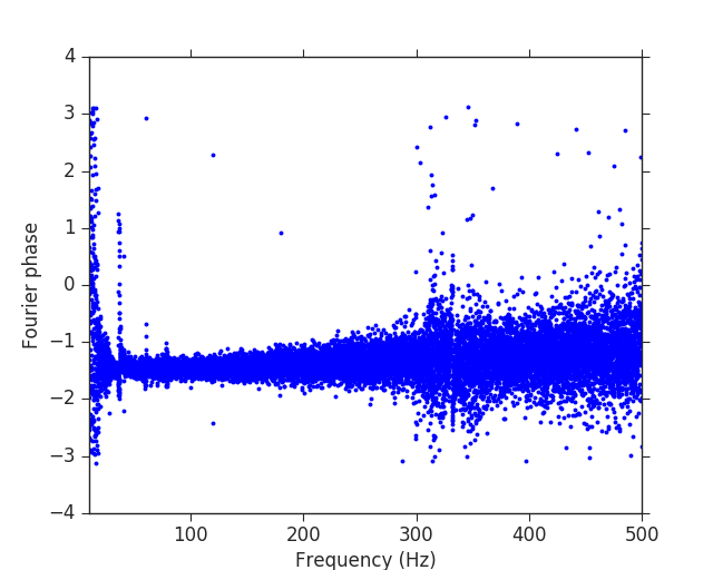
For Gaussian noise we would expect the Fourier phases to be distributed randomly (between -pi and pi). Clearly in the plot shown above, and in Creswell et al., this is not the case. However, the authors overlooked one critical detail here. When you take a Fourier transform of a time series you are implicitly assuming that the data are cyclical (i.e. that the first point is adjacent to the last point). For colored Gaussian noise this assumption will lead to a discontinuity in the data at the two end points, because these data are not causally connected. This discontinuity can be responsible for misleading plots like the one above.

To try to demonstrate this I perform two tests. First I whiten the colored LIGO noise by measuring the power spectral density (see the LOSC example, which I use directly in my ipython notebook, for some background on colored noise and noise power spectral density), then dividing the data in the Fourier domain by the power spectral density, and finally converting back to the time domain. This process will corrupt some data at the edges so after whitening we only consider the middle half of the data. Then we can make the same plot:

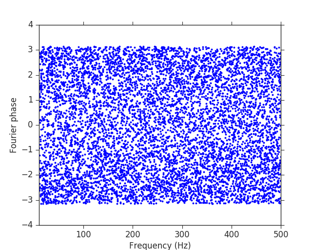
And we can see that there are now no correlations visible in the data. For white Gaussian noise there is no correlation between adjacent points, so no discontinuity is introduced when treating the data as cyclical. I therefore assert that Figure 3 of Creswell et al. actually has no meaning when generated using anything other than whitened data.

I would also like to mention that measuring the noise power spectral density of LIGO data can be challenging when the data are non-stationary and include spectral lines (as Creswell et al. point out). Therefore it can be difficult to whiten data in many circumstances. For the Livingston data some of the spectral lines are still clearly present after whitening (using the methods described in the LOSC example), and then mild correlations are present in the resulting plot (see ipython notebook). This is not indicative of any type of non-Gaussianity, but demonstrates that measuring the noise power-spectral density of LIGO noise is difficult, and, especially for parameter inference, a lot of work has been spent on answering this question.

To further illustrate that features like those seen in Figure 3 of Creswell et al. can be seen in known Gaussian noise I perform an additional check (suggested by my colleague Vivien Raymond). I generate a 128 second stretch of white Gaussian noise (using numpy.random.normal) and invert the whitening procedure employed on the LIGO data above to produce 128 seconds of colored Gaussian noise. Now the data, previously random, are ‘colored’ Coloring the data in the manner I did makes the full data set cyclical (the last point is correlated with the first) so taking the Fourier transform of the complete data set, I see the expected random distribution of phases (again, see the ipython notebook). However, If I select 32s from the middle of this data, introducing a discontinuity as I mention above, I can produce the following plot:

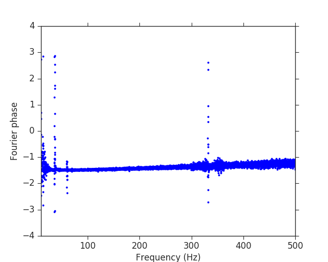
In other words, I can produce an even more extremely correlated example than on the real data, with actual Gaussian noise.

Section III: The data is strongly correlated even after removing the signal

The second half of Creswell et al. explores correlations between the data taken from Hanford and Livingston around GW150914. For me, the main conclusion here is communicated in Figure 7, where Creswell et al. claim that even after removal of the GW150914 best-fit waveform there is still correlation in the data between the two observatories. This is a result I have not been able to reproduce. Nevertheless, if such a correlation were present it would suggest that we have not perfectly subtracted the real signal from the data, which would not invalidate any detection claim. There could be any number of reasons for this, for example the fact that our best-fit waveform will not exactly match what is in the data as we cannot measure all parameters with infinite precision. There might also be some deviations because the waveform models we used, while very good, are only approximations to the real signal (LIGO put out a paper quantifying this possibility). Such deviations might also be indicative of a subtle deviation from general relativity. These are of course things that LIGO is very interested in pursuing, and we have published a paper exploring potential deviations from general relativity (finding no evidence for that), which includes looking for a residual signal in the data after subtraction of the waveform (and again finding no evidence for that).

Finally, LIGO runs “unmodelled” searches, which do not search for specific signals, but instead look for any coherent non-Gaussian behaviour in the observatories. These searches actually were the first to find GW150914, and did so with remarkably consistent parameters to the modelled searches, something which we would not expect to be true if the modelled searches are “missing” some parts of the signal.

With that all said I try to reproduce Figure 7. First I begin by cross-correlating the Hanford and Livingston data, after whitening and band-passing, in a very narrow 0.02s window around GW150914. This produces the following:

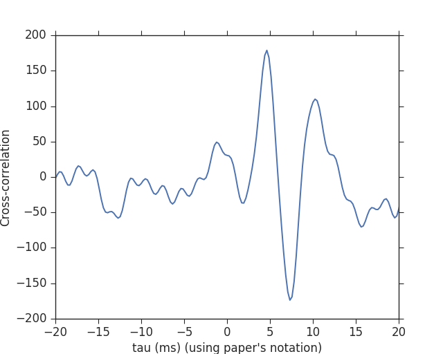
There is a clear spike here at 7ms (which is GW150914), with some expected “ringing” behaviour around this point. This is a much less powerful method to extract the signal than matched-filtering, but it is completely signal independent, and illustrates how loud GW150914 is. Creswell et al. however, do not discuss their normalization of this cross-correlation, or how likely a deviation like this is to occur from noise alone. Such a study would be needed before stating that this is significant—In this case we know this signal is significant from other, more powerful, tests of the data. Then I repeat this but after having removed the best-fit waveform from the data in both observatories (using only products made available in the LOSC example notebooks). This gives:

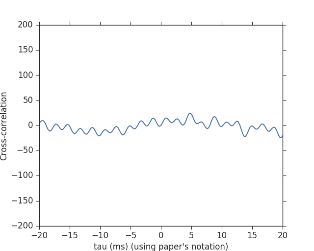
This shows nothing interesting at all.

Section IV: Why would such correlations not invalidate the LIGO detections?

Creswell et al. claim that correlations between the Hanford and Livingston data, which in their results appear to be maximized around the time delay reported for GW150914, raised questions on the integrity of the detection. They do not. The authors claim early on in their article that LIGO data analysis assumes that the data are Gaussian, independent and stationary. In fact, we know that LIGO data are neither Gaussian nor stationary and if one reads through the technical paper accompanying the detection PRL, you can read about the many tests we run to try to distinguish between non-Gaussianities in our data and real signals. But in doing such tests, we raise an important question: “If you see something loud, how can you be sure it is not some chance instrumental artifact, which somehow was missed in the various tests that you do”. Because of this we have to be very careful when assessing the significance (in terms of sigmas—or the p-value, to use the correct term). We assess the significance using a process called time-shifts. We first look through all our data to look for loud events within the 10ms time-window corresponding to the light travel time between the two observatories. Then we look again. Except the second time we look we shift ALL of the data from Livingston by 0.1s. This delay is much larger than the light travel time so if we see any interesting “events” now they cannot be genuine astrophysical events, but must be some noise transient. We then repeat this process with a 0.2s delay, 0.3s delay and so on up to time delays on the order of weeks long. In this way we’ve conducted of order 10 million experiments. For the case of GW150914 the signal in the non-time shifted data was louder than any event we saw in any of the time-shifted runs—all 10 million of them. In fact, it was still a lot louder than any event in the time-shifted runs as well. Therefore we can say that this is a 1-in-10-million event, without making any assumptions at all about our noise. Except one. The assumption is that the analysis with Livingston data shifted by e.g. 8s (or any of the other time shifts) is equivalent to the analysis with the Livingston data not shifted at all. Or, in other words, we assume that there is nothing special about the non-time shifted analysis (other than it might contain real signals!). As well as the technical papers, this is also described in the science summary that accompanied the GW150914 PRL.

Nothing in the paper “On the time lags of the LIGO signals” suggests that the non-time shifted analysis is special. The claimed correlations between the two detectors due to resonance and calibration lines in the data would be present also in the time-shifted analyses—The calibration lines are repetitive lines, and so if correlated in the non-time shift analyses, they will also be correlated in the time-shift analyses as well. I should also note that potential correlated noise sources was explored in another of the companion papers to the GW150914 PRL. Therefore, taking the results of this paper at face value, I see nothing that calls into question the “integrity” of the GW150914 detection.

Section V: Wrapping up

I have tried to reproduce the results quoted in “On the time lags of the LIGO signals”. I find the claims of section 2 are due to an issue in how the data is Fourier transformed, and do not reproduce the correlations claimed in section 3. Even if taking the results at face value, it would not affect the 5-sigma confidence associated with GW150914. Nevertheless I am in contact with the authors and we will try to understand these discrepancies.

For people interested in trying to explore LIGO data, check out the LIGO Open Science Center tutorials. As someone who was involved in the internal review of the LOSC data products it is rewarding to see these materials being used. It is true that these tutorials are intended as an introduction to LIGO data analysis, and do not accurately reflect many of the intricacies of these studies. For the interested reader a number of technical papers, for example this one, accompany the main PRL and within this paper and its references you can find all the nitty-gritty about how our analyses work. Finally, the PyCBC analysis toolkit, which was used to obtain the 5-sigma confidence, and of which I am one of the primary developers, is available open-source on git-hub. There are instructions here and also a number of examples that illustrate a number of aspects of our data analysis methods.

This article was circulated in the LIGO-Virgo Public Outreach and Education mailing list before being made public, and I am grateful to comments and feedback from: Christopher Berry, Ofek Birnholtz, Alessandra Buonanno, Gregg Harry, Martin Hendry, Daniel Hoak, Daniel Holz, David Keitel, Andrew Lundgren, Harald Pfeiffer, Vivien Raymond, Jocelyn Read and David Shoemaker.

A Response to “On the time lags of the LIGO signals” (Guest Post) Read More »

15 Comments

Congratulations to Grant and Jason!

Advising graduate students as they make the journey from learners to working scientists is one of the great pleasures and privileges of academic life. Last week featured the Ph.D. thesis defenses of not one, but two students I’ve been working with, Grant Remmen (who was co-advised by Cliff Cheung) and Jason Pollack. It will be tough to see them go — both got great postdocs, Grant accepting a Miller Fellowship at Berkeley, and Jason heading to the University of British Columbia — but it’s all part of the cycle of life.

Jason Pollack (L), Grant Remmen (R), and their proud advisor.

Of course we advisors love all of our students precisely equally, but it’s been a special pleasure to have Jason and Grant around for these past five years. They’ve helped me enormously in many ways, as we worked to establish a research program in the foundations of quantum gravity and the emergence of spacetime. And along the way they tallied up truly impressive publication records (GR, JP). I especially enjoy that they didn’t just write papers with me, but also with other faculty, and with fellow students without involving professors at all.

I’m very much looking forward to seeing how Jason and Grant both continue to progress and grow as theoretical physicists. In the meantime, two more champagne bottles get added to my bookshelf, one for each Ph.D. student — Mark, Eugene, Jennifer, Ignacy, Lotty, Heywood, Chien-Yao, Kim, and now Grant and Jason.

Congrats!

Congratulations to Grant and Jason! Read More »

7 Comments

The Big Picture: Paperback Day

I presume most readers of this blog have already purchased their copy of The Big Picture: On the Origins of Life, Meaning, and the Universe Itself. If you’re really dedicated, you have the hardback version and the ebook and the audiobook, as well as a few spare copies stashed here and there in case of emergency.

Today we’re happy to announce that you can finally complete your set by purchasing the paperback edition of TBP. The cover is even shinier than before! Paperbacks, as we all know, make great gifts, whether as romantic tokens for the special someone in your life, or gestures of conciliation toward your bitter enemies.

I have to confess that I not only had great fun writing this book, but have been quite gratified by its reception. Of course there were doubters — and regretfully, most of the doubters have seemed to argue against their own preconceptions of what they thought the book would say, rather than what it actually did say. But a good number of people have not only enjoyed the book, but engaged with its ideas in a serious way. Here are some reviews that came out after hardcover publication a year ago:

In case you still aren’t sure what the book is about (it’s about matching the fundamental laws of nature to the world of our everyday experience), here are the brief discussions of the individual sections we had right here on the blog:

  1. Part One: Cosmos
  2. Part Two: Understanding
  3. Part Three: Essence
  4. Part Four: Complexity
  5. Part Five: Thinking
  6. Part Six: Caring

Or if you’re more audiovisually inclined, a talk I gave at LogiCal-LA back in January of this year:

Sean Carrol "The Big Picture - On the Origins of Life, Meaning and the Universe Itself"

Thanks to everyone who has bought the book and engaged with it in thoughtful ways. It’s been a great ride.

The Big Picture: Paperback Day Read More »

43 Comments

Guest Post: Nathan Moynihan on Amplitudes for Astrophysicists

As someone who sits at Richard Feynman’s old desk, I take Feynman diagrams very seriously. They are a very convenient and powerful way of answering a certain kind of important physical question: given some set of particles coming together to interact, what is the probability that they will evolve into some specific other set of particles?

Unfortunately, actual calculations with Feynman diagrams can get unwieldy. The answers they provide are only approximate (though the approximations can be very good), and making the approximations just a little more accurate can be a tremendous amount of work. Enter the “amplitudes program,” a set of techniques for calculating these scattering probabilities more directly, without adding together a barrel full of Feynman diagrams. This isn’t my own area, but we’ve  had guest posts from Lance Dixon and  Jaroslav Trnka about this subject a while back.

But are these heady ideas just brain candy for quantum field theorists, or can they be applied more widely? A very interesting new paper just came out that argued that even astrophysicists — who usually deal with objects a lot bigger than a few colliding particles — can put amplitude technology to good use! And we’re very fortunate to have a guest post on the subject by one of the authors, Nathan Moynihan. Nathan is a grad student at the University of Cape Town, studying under Jeff Murugan and Amanda Weltman, who works on quantum field theory, gravity, and information. This is a great introduction to the application of cutting-edge mathematical physics to some (relatively) down-to-Earth phenomena.


In a recent paper, my collaborators and I (Daniel Burger, Raul Carballo-Rubio, Jeff Murugan and Amanda Weltman) make a case for applying modern methods in scattering amplitudes to astrophysical and cosmological scenarios. In this post, I would like to explain why I think this is interesting, and why you, if you’re an astrophysicist or cosmologist, might want to use the techniques we have outlined.

In a scattering experiment, objects of known momentum p are scattered from a localised target, with various possible outcomes predicted by some theory. In quantum mechanics, the probability of a particular outcome is given by the square of the scattering amplitude, a complex number that can be derived directly from the theory. Scattering amplitudes are the central quantities of interest in (perturbative) quantum field theory, and in the last 15 years or so, there has been something of a minor revolution surrounding the tools used to calculate these quantities (partially inspired by the introduction of twistors into string theory). In general, a particle theorist will make a perturbative expansion of the path integral of her favorite theory into Feynman diagrams, and mechanically use the Feynman rules of the theory to calculate each diagram’s contribution to the final amplitude. This approach works perfectly well, although the calculations are often tough, depending on the theory.

Astrophysicists, on the other hand, are often not concerned too much with quantum field theories, preferring to work with the classical theory of general relativity. However, it turns out that you can, in fact, do the same thing with general relativity: perturbatively write down the Feynman diagrams and calculate scattering amplitudes, at least to first or second order. One of the simplest scattering events you can imagine in pure gravity is that of two gravitons scattering off one another: you start with two gravitons, they interact, you end up with two gravitons. It turns out that you can calculate this using Feynman diagrams, and the answer turns out to be strikingly simple, being barely one line.

The calculation, on the other hand, is utterly vicious. An unfortunate PhD student by the name of Walter G Wesley was given this monstrous task in 1963, and he found that to calculate the amplitude meant evaluating over 500 terms, which as you can imagine took the majority of his PhD to complete (no Mathematica!). The answer, in the end, is breathtakingly simple. In the centre of mass frame, the cross section for this amplitude is:

\frac{d\sigma}{d\Omega} = 4G^2E^2 \frac{\cos^{12}\frac12\theta}{\sin^{4}\frac12\theta}

Where G is Newton’s constant, E is the energy of the gravitons, and \theta is the scattering angle. The fact that they are so cumbersome has meant that many in the astrophysics community may eschew calculations of this type.

However, the fact that the answer is so simple implies that there may be an easier route to calculation than evaluating all 500 diagrams. Indeed, this is exactly what we have tried to allude to in our paper: using the methods we have outlined, this calculation can be done on half a page and with little effort.

The technology that we introduce can be summed up as follows and should be easily recognised as common tools present in any physicists arsenal: a change of variables (for the more mathematically inclined reader, a change of representation), recursion relations and complex analysis. Broadly speaking, the idea is to take the basic components of Feynman diagrams: momentum vectors and polarisation vectors (or tensors) and to represent them as spinors, objects that are inherently complex in nature (they are elements of a complex vector space). Once we do that, we can utilise the transformation rules of spinors to simplify calculations. This simplifies things a bit, but we can do better.

The next trick is to observe that Feynman diagrams all have one common feature: they contain real singularities (meaning the amplitude blows up) wherever there are physical internal lines. These singularities usually show up as poles, functions that behave like 1/z^n. Typically, an internal line might contribute a factor like \frac{1}{p^2 + m^2}, which obviously blows up around p^2 = -m^2.

We normally make ourselves feel better by taking these internal lines to be virtual, meaning they don’t correspond to physical processes that satisfy the energy-momentum condition p^2 = -m^2 and thus never blow up. In contrast to this, the modern formulation insists that internal lines do satisfy the condition, but that the pole is complex. Now that we have complex poles, we can utilise the standard tools of complex analysis, which tells us that if you know about the poles and residues, you know everything. For this to work, we are required to insist that at least some of external momentum is complex, since the internal momentum depends on the external momentum. Thankfully, we can do this in such a way that momentum conservation holds and that the square of the momentum is still physical.

The final ingredient we need are known as the BCFW recursion relations, an indispensable tool used by the amplitudes community developed by Britto, Cachazo, Feng and Witten in 2005. Roughly speaking, these relations tell us that we can turn a complex, singular, on-shell amplitude of any number of particles into a product of 3-particle amplitudes glued together by poles. Essentially, this means we can treat amplitudes like lego bricks and stick them together in an intelligent way in order to construct a really-difficult-to-compute amplitude from some relatively simple ones.

In the paper, we show how this can be achieved using the example of scattering a graviton off a scalar. This interaction is interesting since it’s a representation of a gravitational wave being ‘bent’ by the gravitational field of a massive object like a star. We show, in a couple of pages, that the result calculated using these methods exactly corresponds with what you would calculate using general relativity.

If you’re still unconvinced by the utility of what I’ve outlined, then do look out for the second paper in the series, hopefully coming in the not too distant future. Whether you’re a convert or not, our hope is that these methods might be useful to the astrophysics and cosmology communities in the future, and I would welcome any comments from any members of those communities.

Guest Post: Nathan Moynihan on Amplitudes for Astrophysicists Read More »

6 Comments
Scroll to Top